case 12 · Personal · 2026
FPGA CNN Accelerator — Verilog hand gesture classifier
A three-layer convolutional neural network built entirely in Verilog on a Tang Primer 20K — no CPU, no soft-core, no vendor neural-net IP. A PC webcam streams 96×96 grayscale frames over UART; the FPGA classifies the hand gesture (0–5 fingers) on-chip and reports the result back over UART and on the board LEDs. 84.3% accuracy on 300 real hardware test images, against an 88.1% validation accuracy of the trained model.
↗ github.com/Prateek2174/tang-primer-cnn- FPGA
- Sipeed Tang Primer 20K — Gowin GW2A-18C
- Input
- PC webcam → OpenCV → UART → 96×96 grayscale
- Network
- 3× Conv (3×3) + ReLU + 2×2 MaxPool → GAP → FC
- Weights
- int8 quantization-aware training → on-chip pROM
- Dataset
- 3,547 self-collected images · 6 classes (0–5 fingers)
- Accuracy
- 84.3% measured on FPGA · 88.1% validation (PyTorch)
- Logic
- 9% LUT/ALU/ROM16 · 6% registers · 59% BRAM (binding)
- Toolchain
- Gowin EDA V1.9.11 · PyTorch (training)
What it does
The FPGA runs a complete CNN inference pipeline — from raw pixel input to
classified output — with no processor of any kind involved. A Python script on
the PC captures a webcam frame, resizes it to 96×96 grayscale, and sends it
over UART prefixed with a 0xAA 0x55 sync marker. The FPGA
assembles the frame, runs it through three convolutional layers, a global
average pooling stage, and a fully connected classifier, then sends the
predicted finger count (0–5) back as a single byte and lights the
corresponding LED.
All weights — the convolutional filters, per-filter biases, and FC layer weights — are quantized to int8 and stored in on-chip pROM. The entire inference runs in a single clock domain at 27 MHz (the board's raw oscillator, no PLL) with no off-chip memory.
Pipeline
Each stage feeds the next through on-chip BSRAM scratch buffers:
- UART RX + frame assembly —
uart.vreceives bytes at 115200 baud.uart_frame.vwatches for the0xAA 0x55sync marker, then writes the next 9,216 bytes into the resize BSRAM, centering each pixel (pixel − 128) for signed CNN arithmetic. - CONV1 — 3×3 convolution over 96×96×1 → 48×48×8, folding bias-add, ReLU, and 2×2 max-pool into the same MAC FSM. Output stored in Feature Map A (BSRAM).
- CONV2 — 3×3 over 48×48×8 → 24×24×16, same structure. Output in Feature Map B.
- CONV3 — 3×3 over 24×24×16 → 12×12×32. Output in Feature Map C.
- Global average pooling —
global_avg_pool.vaverages each of the 32 channels in Feature Map C to a single value, producing a 32-element vector. - Classifier —
classifier.vruns a fully connected layer over the 32 GAP outputs and takes the argmax to produce the finger-count class. - Output —
uart_tx.vsends the class byte back to the PC; the top-level also drives one LED per class in one-hot encoding.
| Layer | Kernel | Stride | Padding | Channels | Bias |
|---|---|---|---|---|---|
conv1 | 3×3 | 1 | 1 | 1→8 | yes |
conv2 | 3×3 | 1 | 1 | 8→16 | yes |
conv3 | 3×3 | 1 | 1 | 16→32 | yes |
| max pool (after each conv+ReLU) | 2×2 | 2 | 0 | — | — |
| FC | — | — | — | 32→6 | no |
MAC array design
Rather than instantiating three separate conv engines, I wrote a single
reusable MAC datapath in mac_array.v and time-multiplexed it
across all three conv layers via a conv_layer_sel signal.
The MAC FSM folds bias-add, ReLU, and 2×2 max-pool into its own state
machine — there are no separate pool or ReLU modules in the live pipeline.
conv_acc.v implements the inner 9-tap signed multiply-accumulate
for one conv window; mac_array.v loops over channels and spatial
positions and coordinates writes back to the feature map BSRAMs.
BRAM (59% utilised) is the binding resource, not logic — the three feature maps (48×48×8, 24×24×16, 12×12×32) together require 27 of the 46 available BSRAM blocks.
Weights and quantization
The model was trained in PyTorch with quantization-aware training targeting
int8 weights. After training, weights are extracted, quantized, and written
into Gowin pROM initialization files. weight_rom.v exposes
them as an addressed read interface to the MAC array. Biases are also int8,
stored per filter. The ~4 percentage-point drop from validation accuracy
(88.1%) to real hardware accuracy (84.3%) is accounted for by the fixed-point
rounding in the RTL, confirmed by running the same int8 inference in PyTorch
and getting matching numbers — no hardware bug.
Dataset
3,547 images collected by hand — six classes (0 to 5 fingers), shot against varied backgrounds and lighting, multiple subjects. 85/15 train/val split (3,017 / 530 images). The dataset collection was the longest phase of the project; getting enough variation in background and hand orientation to make the model generalize was what made the final 84.3% on real hardware hold up.
Demo
Design notes
Working notes from the design phase — the CNN datapath structure, BSRAM addressing, and MAC FSM carried forward into the final build.
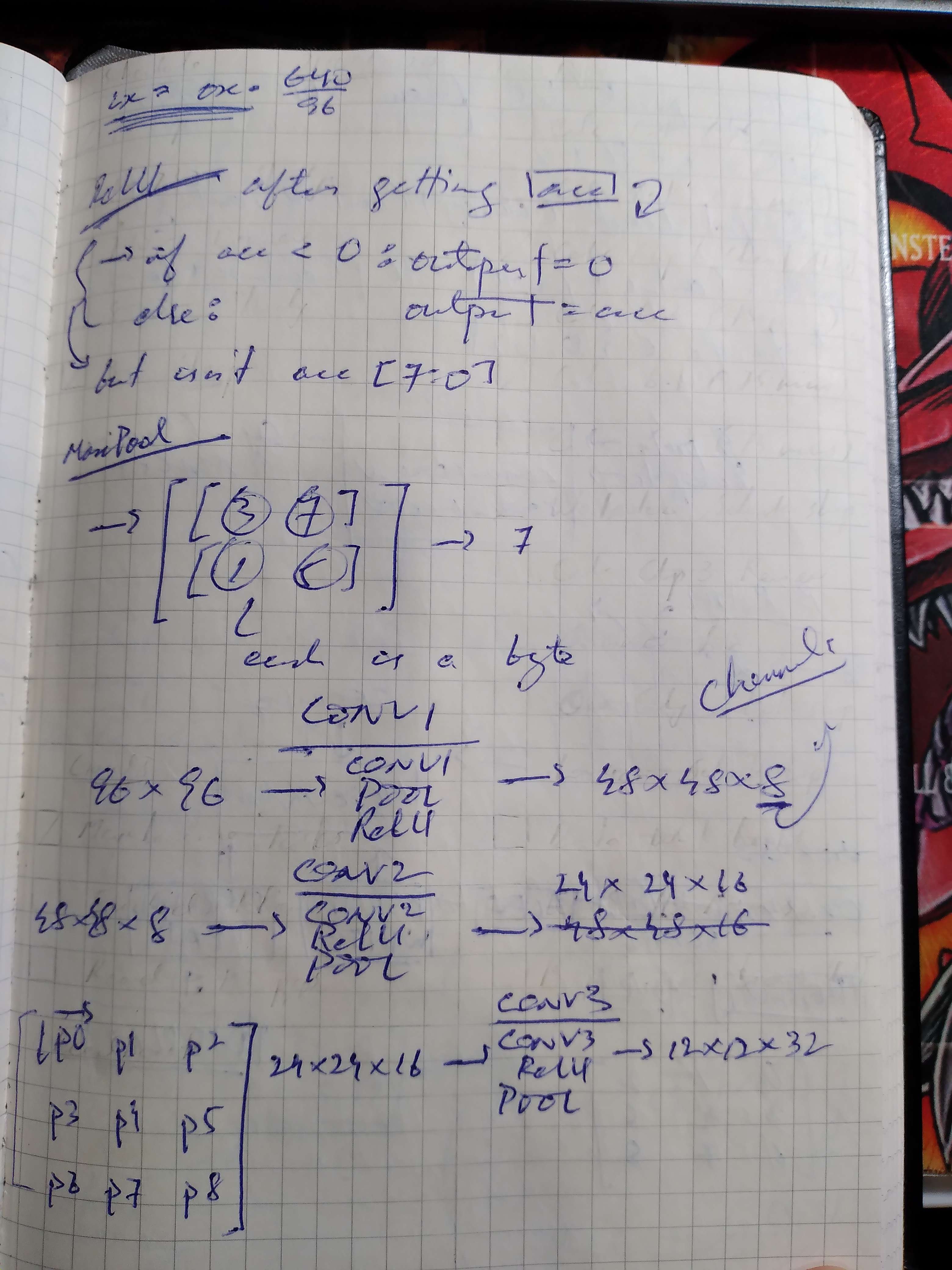
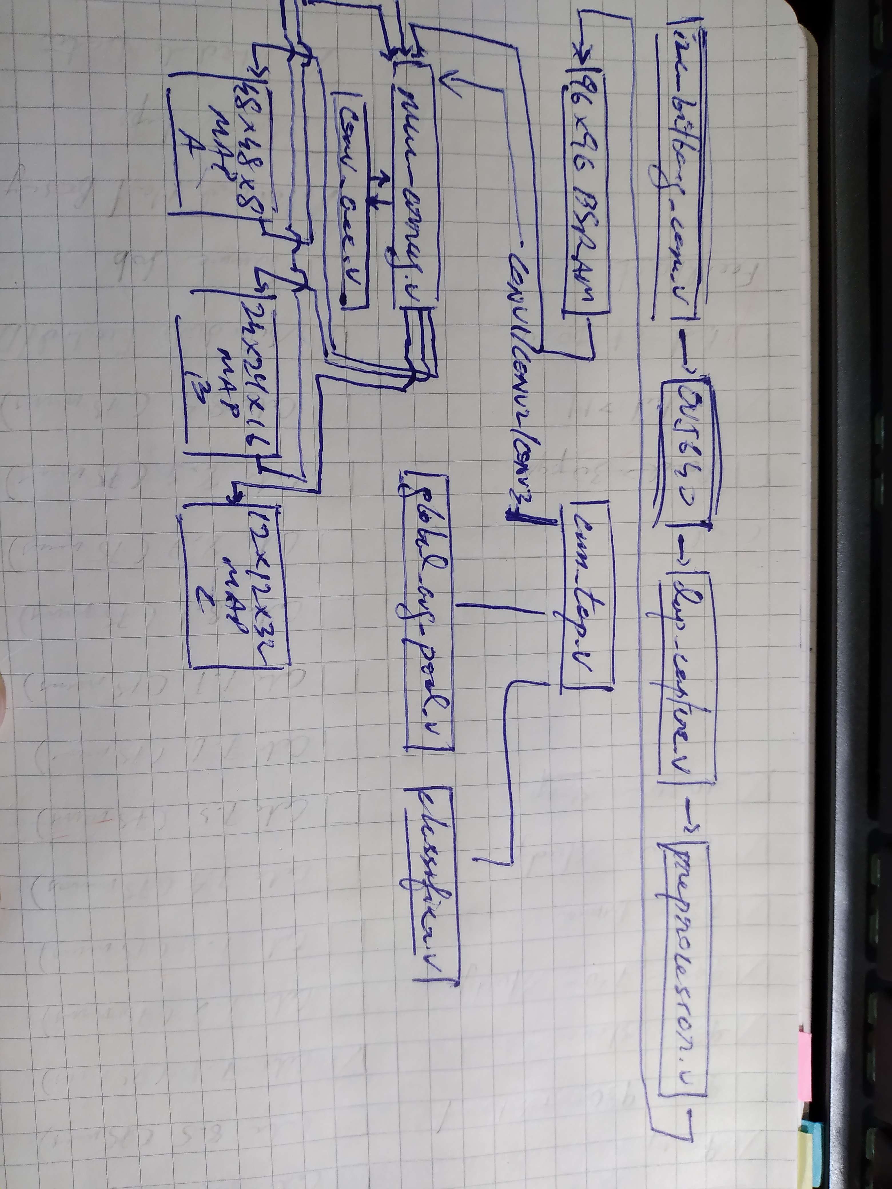
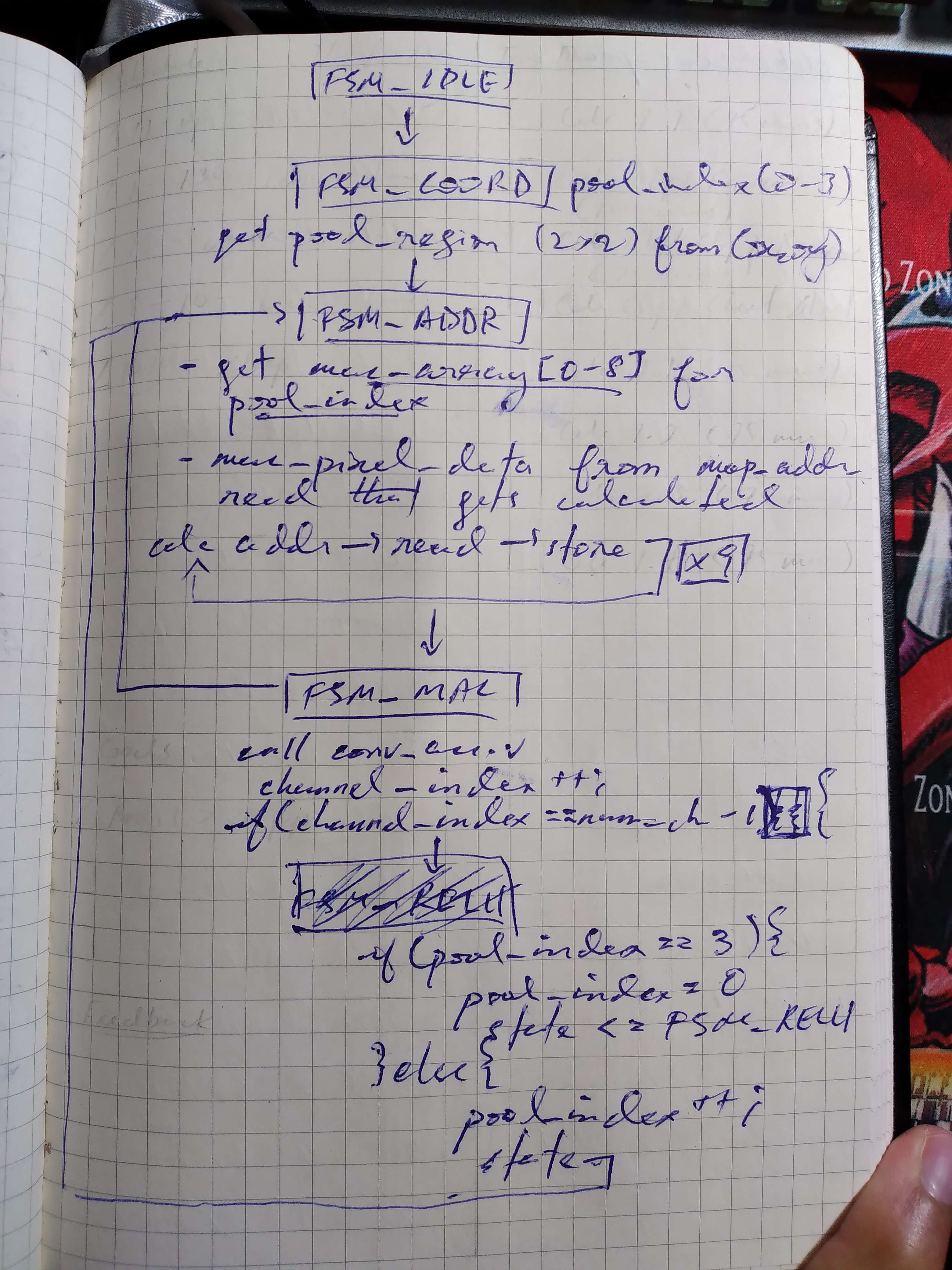
mac_array.v FSM — adds the per-channel accumulate loop and pool-index increment that made it into the final implementation.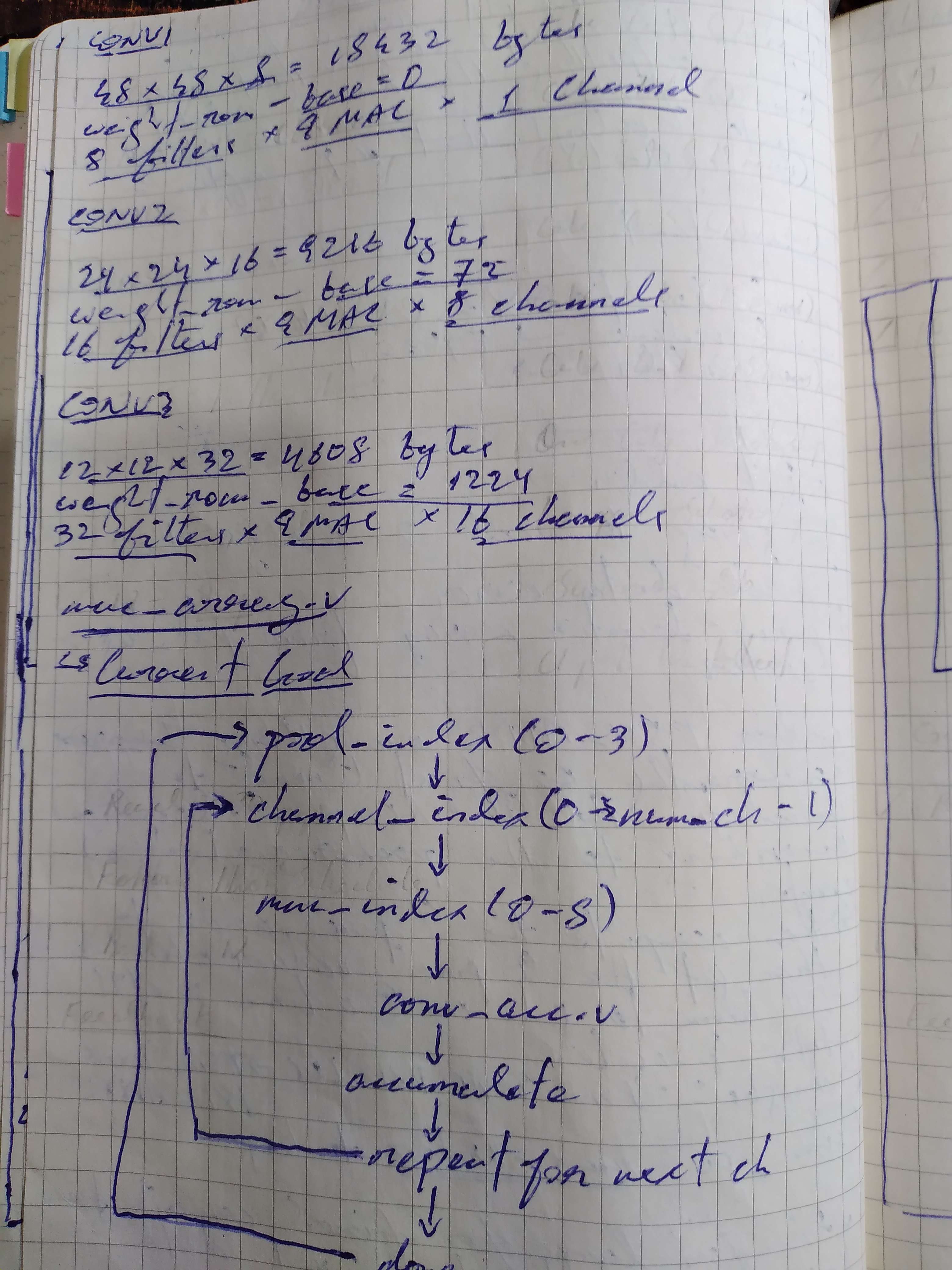
What was hard
The biggest challenge was fitting the feature maps in BRAM. At 59% utilisation BRAM was the binding resource — logic sat at 9%. The three feature map buffers (48×48×8, 24×24×16, 12×12×32) together consume 27 of the 46 available BSRAM blocks. Getting the addressing right — the conv window slides across two spatial dimensions and a channel dimension simultaneously — required careful indexing math to avoid BSRAM port conflicts and to keep the MAC loop on schedule.
The earlier design fed a live OV5640 camera directly into the FPGA over a DVP parallel interface, but that path had frame-sync and decimation complexity that was adding noise to the debugging. Switching to UART from a PC webcam gave full control over the input — exact pixel values, known frame boundaries, reproducible test images — which is what made the cycle-accurate simulation vs. hardware accuracy comparison possible.
Quantization-aware training was necessary. Naively quantizing a float32-trained model to int8 post-hoc dropped accuracy below 70%. Retraining with QAT and re-quantizing recovered it to 88.1% val / 84.3% hardware.
What's next
- Live camera input — restore the OV5640 DVP path now that the CNN datapath is stable; eliminates the PC middleman and makes the system fully self-contained
- Pipeline parallelism — the current design processes one conv layer at a time sequentially; overlapping CONV2 with CONV1's output write-back would cut latency
- More classes — extend beyond 0–5 fingers to ASL letters or other gestures; requires a larger dataset and more filters (wider network), which will push BRAM usage past 100% and force a CONV3 feature map compression strategy
- On-chip display output — drive an HDMI or SPI display directly from the FPGA showing the classified gesture alongside the confidence scores, without needing the UART return path to a PC